42 pivot table row labels not showing
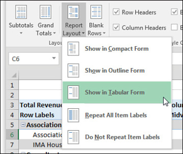
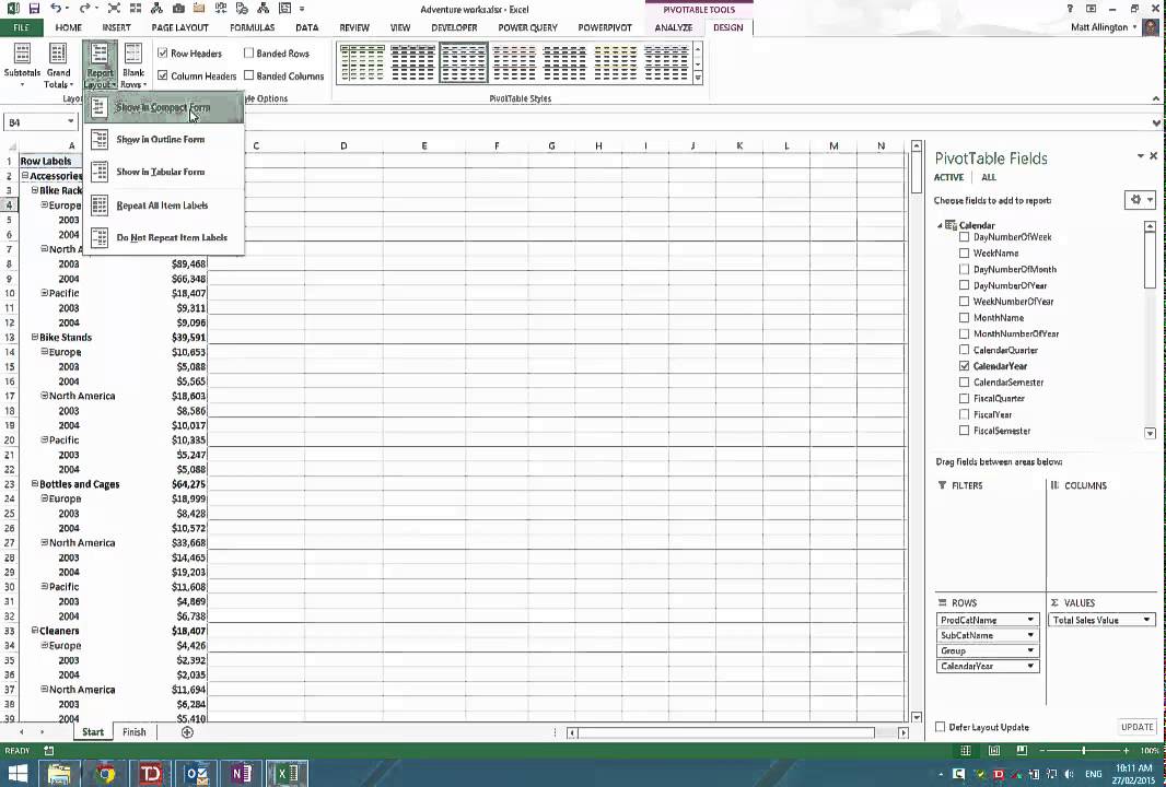
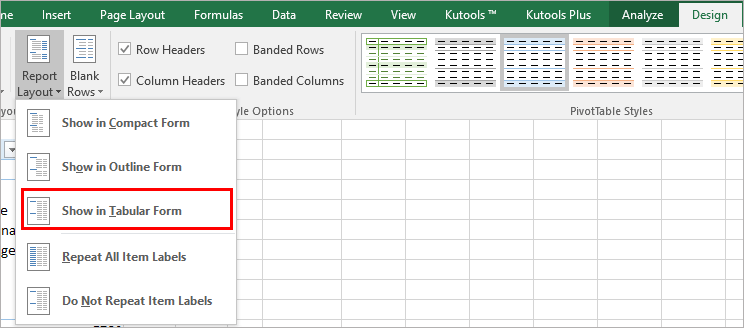
101 Advanced Pivot Table Tips And Tricks You Need To Know 25/04/2022 · In this example, if we were to add data past Row 51 or Column I our pivot table would not include it in the results. To create and name your table. Select your data. Go to the Insert tab and press the Table button in the Tables section, or use the keyboard shortcut Ctrl + T. Press the OK button. With the active cell inside the table, go to the Table Tools Design tab. … › xlpivot05Fix Excel Pivot Table Missing Data Field Settings Aug 31, 2022 · To show the item labels in every row, for all pivot fields: Select a cell in the pivot table; On the Ribbon, click the Design tab, and click Report Layout; Click Repeat All Item Labels; To show the item labels in every row, for a specific pivot field: Right-click an item in the pivot field; In the Field Settings dialog box, click the Layout ...
Pivot table rows Indented & unable to un-indent 3 measures in my Values field in Excel pivot table but 2 of the Measure labels are indented & I cannot correct it back to standard layout (no indent) excel. pivot-table. Share. asked Sep 12 at 3:36. Mturks83. 79 2 8. Add a comment.

Pivot table row labels not showing
Trap and fix errors in your VLOOKUP in Google Sheets - Ablebits.com If you use relative cell references (e.g. A1) instead of absolute ones (e.g. $A$1) and then modify the table (e.g. add a column), the data will shift, the references will change, and the formula will refer to wrong cells: I added the "ID" column. The "Price" column is not included in the range anymore, thus the price cannot be found. 50 Keyboard Shortcuts in Excel You Should Know in 2022 - Simplilearn.com Alt + Shift + Left arrow. Now that we have looked at the different shortcut keys for formatting cells, rows, and columns, it is time to jump into understanding an advanced topic in Excel, i.e. dealing with pivot tables. Let's look at the different shortcuts to summarize your data using a pivot table. Pivot chart ( Note: this change is not optional. No help to be offered until this moderation request has been fulfilled.) 1. Use code tags for VBA. [code] Your Code [/code] (or use the # button) 2. If your question is resolved, mark it SOLVED using the thread tools 3. Click on the star if you think someone helped you Regards Ford Register To Reply
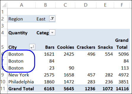
Pivot table row labels not showing. Inerface for viewing specific data from a table If your data are in a table, the headers (field names) should already have filter drop down arrows. If not, click in any of the headers of your data and select Sort & Filter > Filter on the home tab of the ribbon. You can easily use the filter arrows to sort and filter the data. When you're done, select Sort & filter > Clear to show all data again. techcommunity.microsoft.com › t5 › excelPivot Table - Date - Group by Month does not work May 07, 2019 · @Detlef Lewin I was trying to apply your solution, when suddenly the pivot table itself divided my date into months: The problem is, I have no idea how I did this. the original table only has 'Date' (not months). He added the field 'month' himself. It is perfect, because this is exactly what I need. (with this, I don't need to group). Tableau Essentials: Formatting Tips - Tooltips - InterWorks As an example, inserting the data update time will add the field into the tooltip text box, showing your users when the data source connection was last refreshed. Finally, the last button (X) is the Clear Formatting button which will wipe all of the style selections from the tooltip. This will not erase your measures or text, just the formatting. What is a Pivot Table? Definition from WhatIs.com pivot table: A pivot table is a program tool that allows you to reorganize and summarize selected columns and rows of data in a spreadsheet or database table to obtain a desired report. A pivot table doesn't actually change the spreadsheet or database itself. In database lingo, to pivot is to turn the data (see slice and dice ) to view it from ...
changing Date format in a pivot table - Microsoft Tech Community 04/03/2019 · @Jan Karel PieterseI have a pivot table and chart in (current) Office 365 with dates in the row column; when I follow the same steps as described below, there is no "Number Format" button showing in the Field Settings dialog - see screen copy below.Why is that? I managed to change the date format within the pivot table (using "ungroup"), but this new … PBI Theming JSON - Missing Properties - Microsoft Power BI Community Example: matrix visual (pivot table) Column grand total; Row grand total; Example: slicer visual. Values --> border postion (top, bottom, left, right) Another area are the already matured new shapes. The former attribute "shape" does not work with these anymore or many of the new fetures are not available to define, respectively. How to display multiple subtotal rows in a Microsoft ... - TechRepublic Instead, do the following: Click any cell in the Region column in the PivotTable. Click the contextual PivotTable Analyze tab. In the Active Field group, click Field Settings. In the resulting ... Open a Microsoft Excel file with pivot tables in Numbers on iPhone ... You can open an Excel file with pivot tables in Numbers on iPhone, iPad, and Mac: To open an Excel file with Numbers on your iPhone or iPad, tap the file in the spreadsheet manager in Numbers. If you don't see the spreadsheet manager, tap the Back button (on an iPhone) or tap Spreadsheets (on an iPad), then tap the Excel file that you want to open.
5 Ways To Fix Excel Cell Contents Not Visible Issue Select a cell or cell range where the text is not showing up. Right-click on the selected cell or cell range and click Format Cells. From the pop-up window, click on the Font tab and then change the default font (usually Calibri) to any other font, like 'Arial' or 'Times New Roman'. Press the OK button. Figure 4 - Format Cells Window Excel Pivot Table Subtotals - Contextures Excel Tips 01/02/2022 · In a new pivot table, when you add fields to the Row Labels area, subtotals are automatically shown at the top of each group of items, for the outer fields. You canmove the subtota ls to the bottom of the group, if you prefer. To move the subtotals, follow these steps. Select a cell in the pivot table, and on the Ribbon, click the Design tab. In the Layout group, … Pivot Table- Coloring alternate row - Sisense Community I have a pivot table with only rows and need to give background color to alternate rows. I've uploaded screenshots of existing and required pivot table. Thank you in advance! Labels: Dashboards & Reporting. Required Pivot.png. 157 KB. Pivot Table - Date - Group by Month does not work 07/05/2019 · @Detlef Lewin I was trying to apply your solution, when suddenly the pivot table itself divided my date into months: The problem is, I have no idea how I did this. the original table only has 'Date' (not months). He added the field 'month' himself. It is perfect, because this is exactly what I need. (with this, I don't need to group). However ...
google sheets - How to make Pivot Table repeat row labels ...
3 Ways to Preserve 'Percent of Total' within Filtered Dimensions Step 1: Right-click the data source and select duplicate (break any active links from primary to secondary). Step 2: Build out your primary data source (based on the view above). Step 3: Create a calculated field called % of Total: 1 SUM (primary [Sales]) / SUM (secondary [Sales]). Step 4: Format the calculated field to show a percentage.
Show all items with no data on rows / columns in Pivot Table ...
support.google.com › datastudio › answerPivot table reference - Data Studio Help - Google Example pivot table showing revenue per user, by country, quarter, and year. This table easily summarizes the data from the previous example. You can also quickly spot outliers or anomalies in your data. Notice that several countries had no revenue in Q4, for example. Pivot tables in Data Studio support adding multiple row and column dimensions.
How to Hide, Replace, Empty, Format (blank) values with an ...
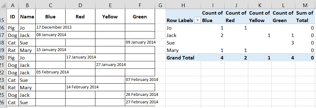
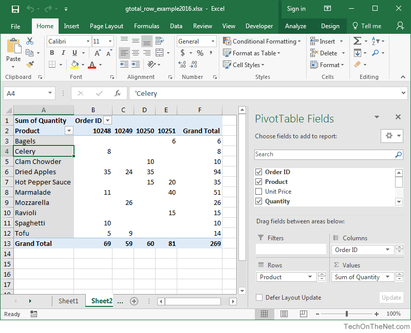
How To Compare Multiple Lists of Names with a Pivot Table Column E of the Pivot Table contains the Grand Total (sum of columns B:D). People that volunteered all three years will have a “3” in column E. We should sort the pivot table so all the people with a “3” in column E appear at the top of the list. This will …

How to make row labels on same line in pivot table?
› pivot-table-tips-and-tricks101 Advanced Pivot Table Tips And Tricks You Need To Know Apr 25, 2022 · Without a table your range reference will look something like above. In this example, if we were to add data past Row 51 or Column I our pivot table would not include it in the results. To create and name your table. Select your data. Go to the Insert tab and press the Table button in the Tables section, or use the keyboard shortcut Ctrl + T.
Making Report Layout Changes | Customizing a Pivot Table in ...
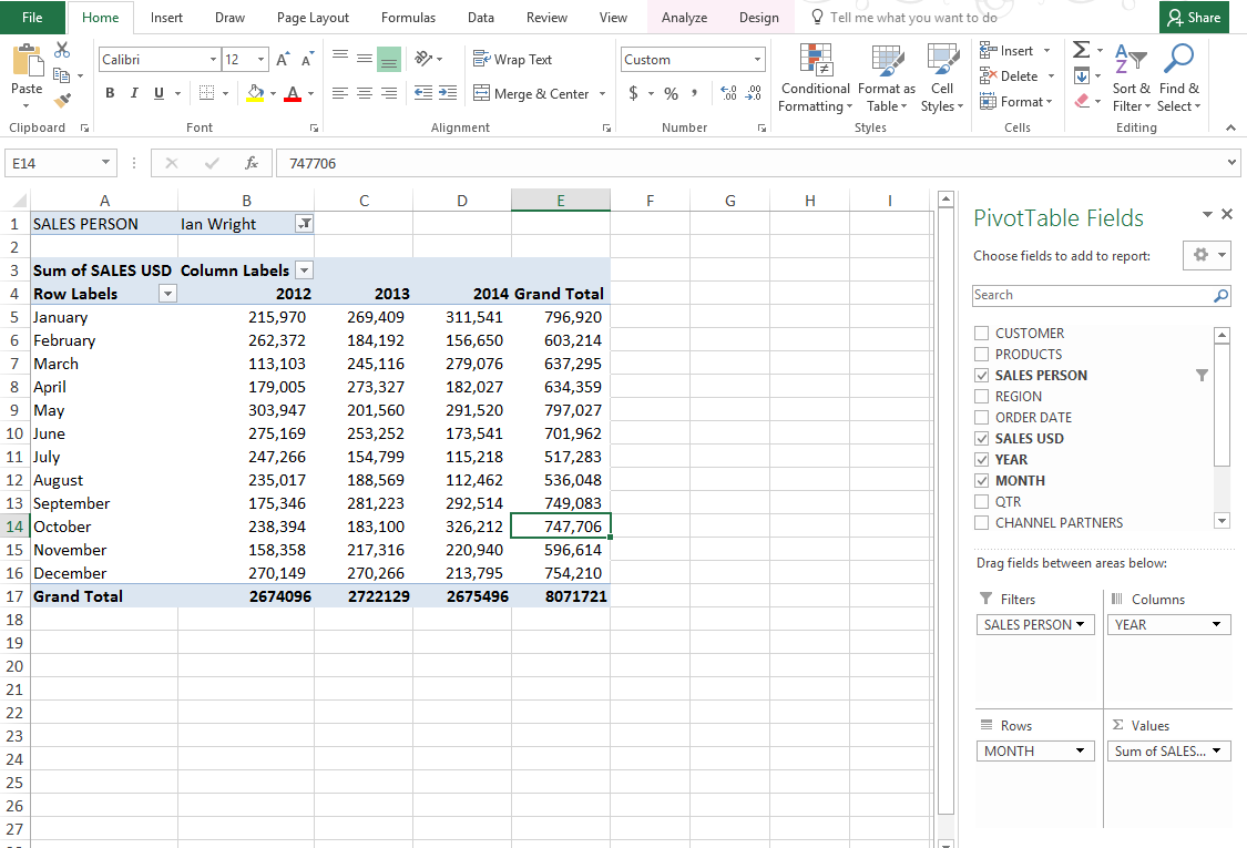
en.wikipedia.org › wiki › Pivot_tablePivot table - Wikipedia Row labels are used to apply a filter to one or more rows that have to be shown in the pivot table. For instance, if the "Salesperson" field is dragged on this area then the other output table constructed will have values from the column "Salesperson", i.e. , one will have a number of rows equal to the number of "Sales Person".
Top 3 Excel Pivot Table Issues Resolved | MyExcelOnline
multiple pivot tables in the same sheet using apache poi One could calculate the rows per pivot table as follows: 4 rows at top for possible report filters 1 row per unique item per row label, multiple row labels multiply unique items 1 row for the heading of col labels 1 row for the heading of column labels having data consolidate functions 1 row for the totals

How to Resolve Duplicate Data within Excel Pivot Tables ...
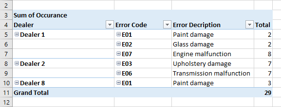
How to Make a Pie Chart in Excel & Add Rich Data Labels to ... - ExcelDemy Creating and formatting the Pie Chart. 1) Select the data. 2) Go to Insert> Charts> click on the drop-down arrow next to Pie Chart and under 2-D Pie, select the Pie Chart, shown below. 3) Chang the chart title to Breakdown of Errors Made During the Match, by clicking on it and typing the new title.
How to Flatten and repeat Row Labels in a Pivot Table
How to convert rows to columns in Excel (transpose data) - Ablebits.com To switch rows to columns, performs these steps: Select the original data. To quickly select the whole table, i.e. all the cells with data in a spreadsheet, press Ctrl + Home and then Ctrl + Shift + End. Copy the selected cells either by right clicking the selection and choosing Copy from the context menu or by pressing Ctrl + C.
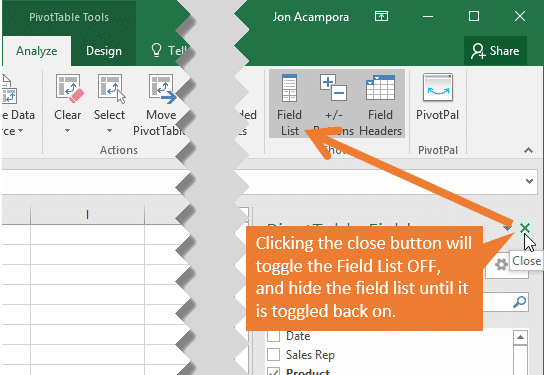
Pivot Table Field List Missing? How to Get It Back - Excel Campus
How to pivot a table (created using DAX-SUMMARIZED, not Power Query) on ... According to your description, you want to pivot a table (created using DAX-SUMMARIZED, not Power Query) on a column. Right? Here are the steps you can follow: (1)This is my test data: ' Test ' (2) We can click " New Table " and enter DAX : Table = ADDCOLUMNS( SUMMARIZE('Test','Test'[GATEGORY]) ,

Pivot table row labels side by side – Excel Tutorials
Fix Excel Pivot Table Missing Data Field Settings - Contextures … 31/08/2022 · In Excel 2010, and later versions, you change a field setting so that the item labels are repeated in each row. This feature does not work if the pivot table is in Compact Layout, so change to Outline form or Tabular form, if necessary, before following the rest of the steps. To change the report layout: Select a cell in the pivot table

How to Replace Blank Cells with Zeros in Excel Pivot Tables
Pivot table enhancements - EPPlus Software EPPlus 5.4 adds support for pivot table filters, calculated columns and shared pivot table caches. The following filters are supported. Item filters - Filters on individual items in row/column or page fields. Caption filters (label filters) - Filters for text on row and column fields. Date, numeric and string filters - Filters using various ...
Pivot table not showing Row Total - Microsoft Community
Pivot columns - Power Query | Microsoft Learn To pivot a column. Select the column that you want to pivot. On the Transform tab in the Any column group, select Pivot column.. In the Pivot column dialog box, in the Value column list, select Value.. By default, Power Query will try to do a sum as the aggregation, but you can select the Advanced option to see other available aggregations.. The available options are:
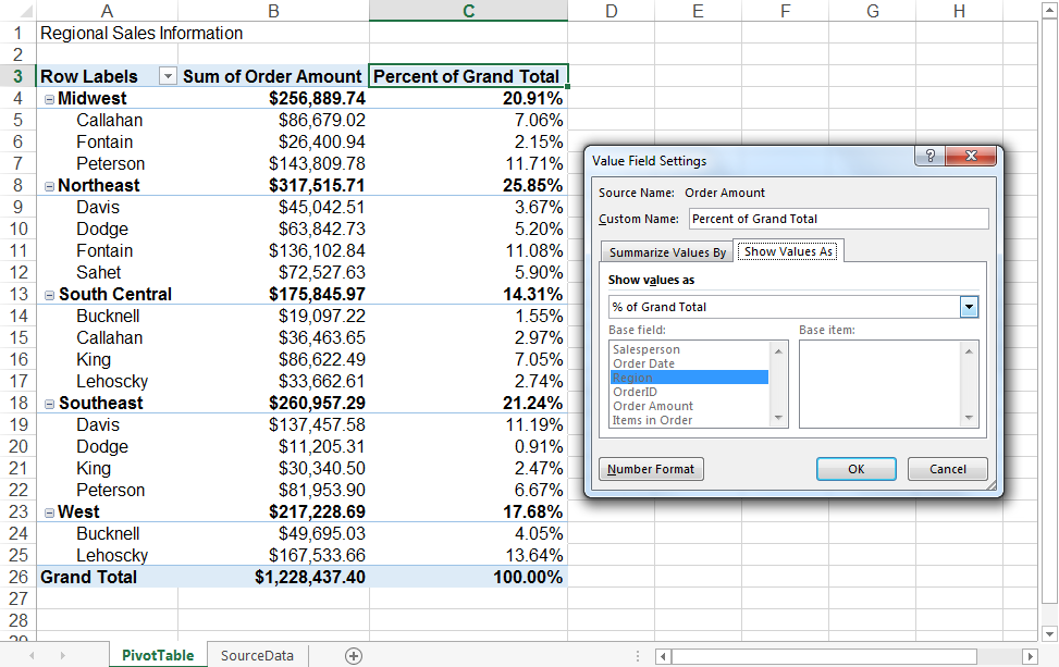
Pivot Table: Percentage of Total Calculations in Excel ...
Consolidate Multiple Worksheets into Excel Pivot Tables To do that, click a value in the Row Labels area and then on the Analyze contextual tab of the ribbon, which is already selected. Now we will modify the value in the Active Field box. It currently says Row, and clicking in the box selects it. These are the products, so we will type in Product and press Enter.
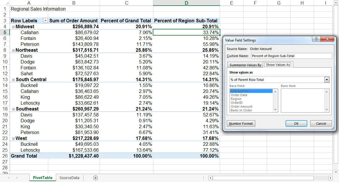
Pivot Table: Percentage of Total Calculations in Excel ...
› definition › pivot-tableWhat is a Pivot Table? Definition from WhatIs.com pivot table: A pivot table is a program tool that allows you to reorganize and summarize selected columns and rows of data in a spreadsheet or database table to obtain a desired report. A pivot table doesn't actually change the spreadsheet or database itself. In database lingo, to pivot is to turn the data (see slice and dice ) to view it from ...
MS Excel 2016: How to Remove Row Grand Totals in a Pivot Table
Group days into months on Sales table? - excelforum.com Group in Years and Months, rename the row label "<29/08/22" and move it down to the last row. Attached Files Monthly Invoice .xlsx (25.1 KB, 4 views) Download
101 Advanced Pivot Table Tips And Tricks You Need To Know ...
How to Hide Zero Values in Excel Pivot Table (3 Easy Methods) 11/08/2022 · If you want to hide zero values from the pivot table quickly, you can definitely make this your go-to method. We can filter the zero values from the Filter field. Just follow these steps to perform this: 📌 Steps. ① First, click on the pivot table that you created from the dataset. ② Now, on the right side, you will see pivot table fields.
MS Excel Pivot Table Deleted Items Remain - Excel and Access
How to Create Pivot Table in Excel: Beginners Tutorial - Guru99 Click on the select table/range button as shown in the image above You will get the following mini window Click in cell address A1 Press Ctrl + A on the keyboard to select all the data cells Your mini window shown now appear as follows Click on Close button to get back to the options window Click on OK button Select the following fields CompanyName
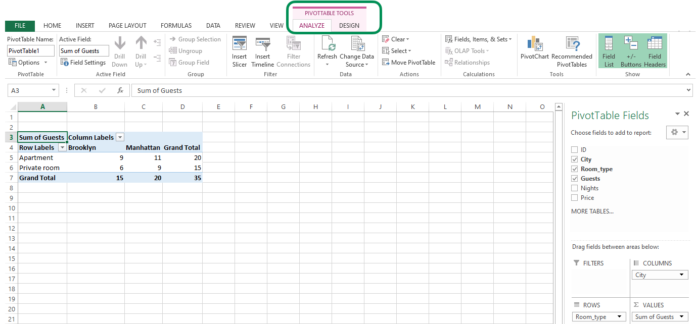
The Pivot table tools ribbon in Excel
Table Header Lookup - Microsoft Tech Community My formula in cell K5 seems to half work. It does show the cheapest price if one of the duplicate postcode rows has all values above zero. (As shown with a postcode starting with CO, but if you use BB it shows a zero). So if all the rows have at least one zero value, then it always returns zero. Part 2 - show column header).
Why is there no Data in my PivotTable? – Kepion Support Center
Pivot table reference - Data Studio Help - Google Example pivot table showing revenue per user, by country, quarter, and year. This table easily summarizes the data from the previous example. You can also quickly spot outliers or anomalies in your data. Notice that several countries had no revenue in Q4, for example. Pivot tables in Data Studio support adding multiple row and column dimensions ...

Fix Excel Pivot Table Missing Data Field Settings
Add an expand or collapse action to a paginated report - Microsoft ... In report design view, click the table or matrix to select it. The Grouping pane displays the row and column groups. If the Grouping pane does not appear, click the View menu and then click Grouping. Right-click anywhere in the title bar of the Grouping pane, and then click Advanced. The Grouping pane mode toggles to show the underlying display ...
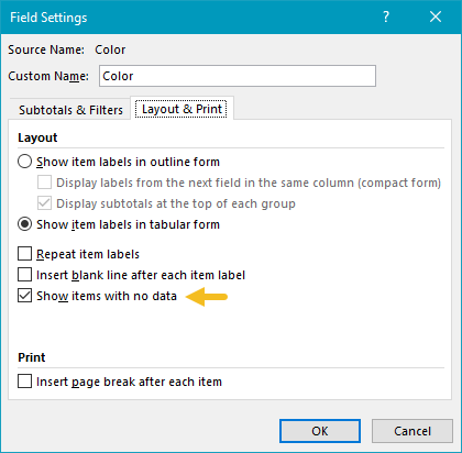
Pivot Table: Pivot table display items with no data | Exceljet
Displaying Row and Column Labels (Microsoft Excel) If your worksheet becomes quite large, it is not unusual for the row and column labels to scroll off the screen so that you can no longer see them. To keep row and column labels visible, consider "freezing" the rows and columns in which the labels are located.
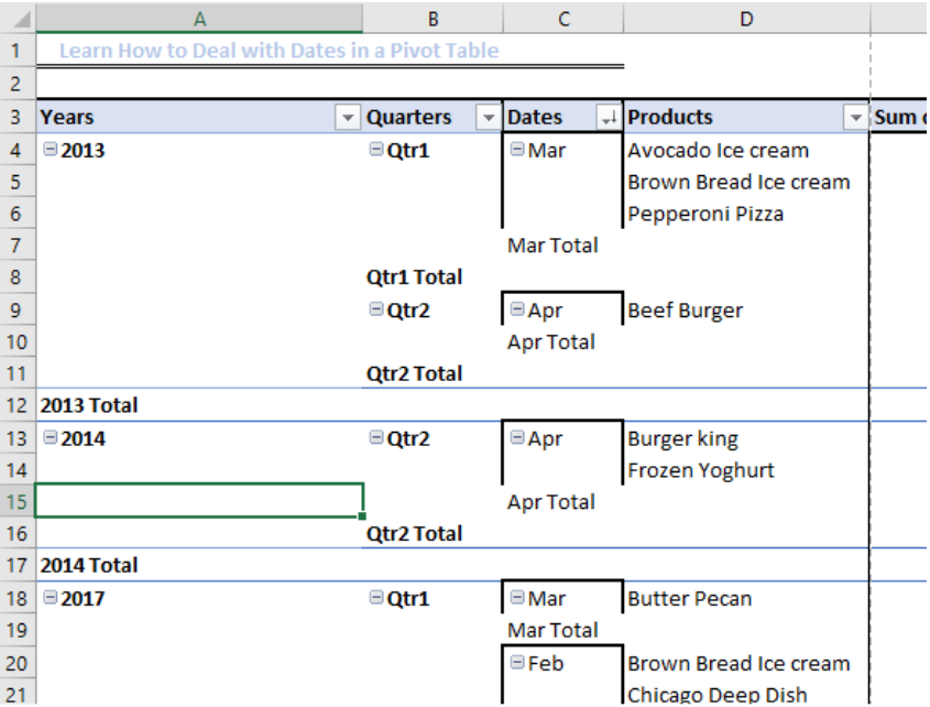
Learn How to Deal with Dates in a Pivot Table | Excelchat
Pivot table - Wikipedia A pivot table usually consists of row, column and data (or fact) fields.In this case, the column is ship date, the row is region and the data we would like to see is (sum of) units.These fields allow several kinds of aggregations, including: sum, average, standard deviation, count, etc.In this case, the total number of units shipped is displayed here using a sum aggregation.
Pivot Table shows row labels instead of field name
How to get the names (titles or labels) of a pandas data ... - Moonbooks Get the row names of a pandas data frame. Let's consider a data frame called df. to get the row names a solution is to do: >>> df.index Get the row names of a pandas data frame (Exemple 1) Let's create a simple data frame:
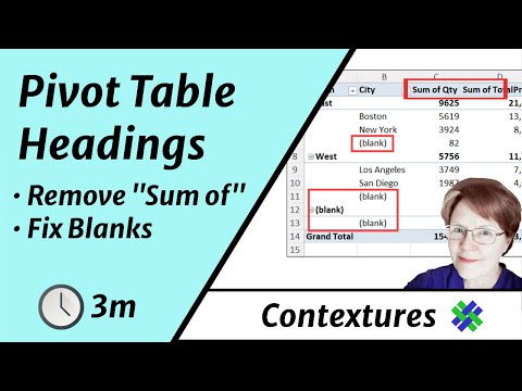
Change Pivot Table Sum of Headings and Blank Labels
› excel-pivot-table-subtotalsExcel Pivot Table Subtotals - Contextures Excel Tips Feb 01, 2022 · In the pivot table shown below, Service is in the Row Labels area, Lead Tech is in the Column Labels area, and Labor Cost is in the Values area. Because Service is the only field in the Row Labels area, it has no subtotal. Multiple Row Fields. When you add another field to the Row Labels area, a subtotal is automatically created for the first ...
How to make row labels on same line in pivot table?
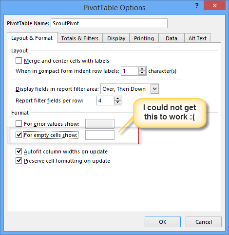
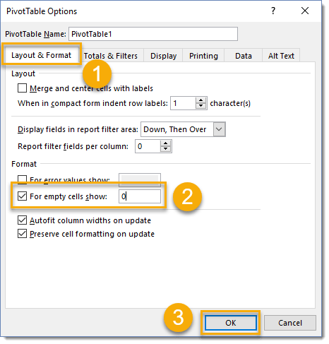
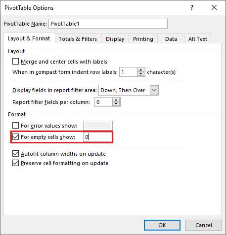
How to Remove Blank Rows in Excel Pivot Table (4 Methods) In the pivot table chart, place your cursor and right-click on the mouse to show pivot table options. Select the " PivotTable Options ". Step 2: A new window will appear. Choose " Layout & Format ". Fill up with " 0 " in the " For empty cells show " option. This will input 0 for every blank cell in the pivot table. Press OK.
Duplicate Items Appear in Pivot Table | Excel Pivot Tables
Pivot Table FAQs and Pivot Chart FAQs - Contextures Excel Tips How do I hide or show the labels on the Pivot Chart? With the pivot chart selected: On the Excel Ribbon, click the Analyze tab. Click the Field Buttons command, to hide/show the PivotChart Field buttons. OR, click the Field Buttons arrow, and select one of the display options. How can I create a Normal chart from pivot table data?
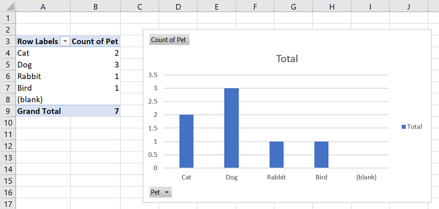
Excel 2016 – How to exclude (blank) values from pivot table
Pivot chart ( Note: this change is not optional. No help to be offered until this moderation request has been fulfilled.) 1. Use code tags for VBA. [code] Your Code [/code] (or use the # button) 2. If your question is resolved, mark it SOLVED using the thread tools 3. Click on the star if you think someone helped you Regards Ford Register To Reply
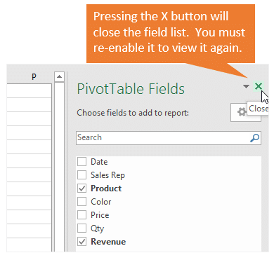
Pivot Table Field List Missing? How to Get It Back - Excel Campus
50 Keyboard Shortcuts in Excel You Should Know in 2022 - Simplilearn.com Alt + Shift + Left arrow. Now that we have looked at the different shortcut keys for formatting cells, rows, and columns, it is time to jump into understanding an advanced topic in Excel, i.e. dealing with pivot tables. Let's look at the different shortcuts to summarize your data using a pivot table.

Fix Excel Pivot Table Missing Data Field Settings
Trap and fix errors in your VLOOKUP in Google Sheets - Ablebits.com If you use relative cell references (e.g. A1) instead of absolute ones (e.g. $A$1) and then modify the table (e.g. add a column), the data will shift, the references will change, and the formula will refer to wrong cells: I added the "ID" column. The "Price" column is not included in the range anymore, thus the price cannot be found.

Automatic Row And Column Pivot Table Labels
Excel 2016 – How to exclude (blank) values from pivot table
excel - PivotTable to show values, not sum of values - Stack ...

Why is there no Data in my PivotTable? – Kepion Support Center
Pivot table row labels side by side – Excel Tutorials

Creating Pivot Tables in Excel for Exported Data – Teaching ...

Repeat Pivot Table row labels • AuditExcel.co.za Pivot Tables ...

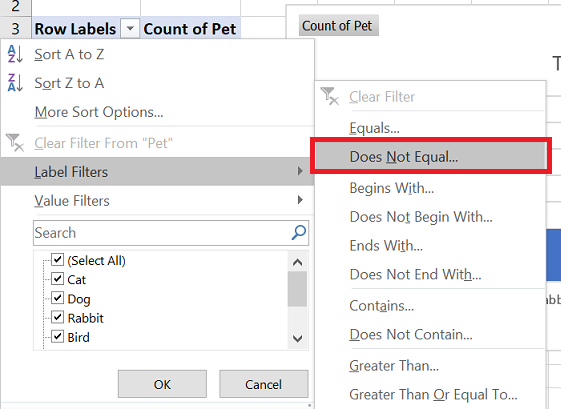
How to Use Label Filters for Text in the Pivot Table? - MS ...

Repeat Pivot Table row labels • AuditExcel.co.za Pivot Tables ...
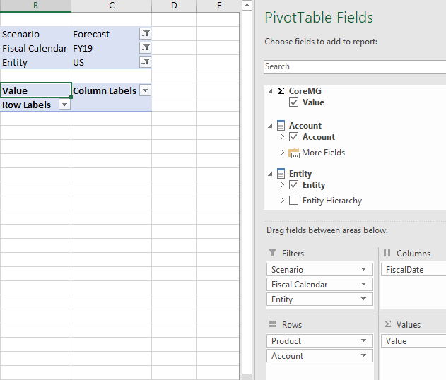
Why is there no Data in my PivotTable? – Kepion Support Center

Pivot Table Defaults to Count Instead of Sum & How to Fix It ...

Excel Pivot Table Subtotals
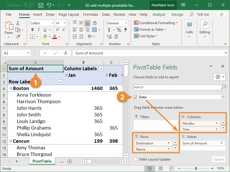
Add Multiple Columns to a Pivot Table | CustomGuide
Post a Comment for "42 pivot table row labels not showing"